python with conda
A very short guide for installing python packages (pymol in this example) as a non-privileged
| Molecular Modeling Lab |
Go to the SECOND part of the Tutorial Go to the FOURTH part of the Tutorial
In the previous section you edited the plumed-common.dat file containing the definition of all the CVs. We now need to set the parameters of the Gaussian hills that are going to be deposited during the metadynamics simulation; namely:
For the sake of simplicity, exception made for the width of the hills "w", in this tutorial all of the other parameters have been already set to standard values.
For additional details, please refer to the official PLUMED tutorials available here.
The width of the hills (one for each CV) needs to be chosen by analysing the evolution of the CV along an unbiased MD simulation. In particular, it is customary to set these values to be roughly between 1/4 and 1/2 of the average fluctuations (standard deviation) of a CV during a short plain MD run [1,2,3].
For this tutorial, we are going to calculate the standard deviation of the CVs over 500 frames spaced 1 ps from each other.
To this aim, we'll use the tool driver of the PLUMED package, requiring:
Driver will read the trajectory and print, for each frame, the values of the CVs specified in the input file (plumed_driver.dat). This file is identical to the file plumed-common.dat, that you have already prepared, apart for an additional line with the instruction to print the CVs values. You can find a copy of this file in the tutorial_files directory.
Copy the input file plumed_driver.dat from the folder tutorial_files/Driver to the folder /EDES/MD/plain/analysis:
cp ../../tutorial_files/Driver/plumed_driver.dat analysis/
cd analysis
Have a look at the file plumed_driver.dat with your favourite text editor (I like emacs: emacs -nw plumed_driver.dat) and compare it with the file plumed-common.dat. You will notice that the only difference is represented by the last line in the plumed_driver.dat file, which contains the PRINT instruction. You can find additional details on the driver tool at PLUMED manual.
Now you can use driver to analyse the unbiased MD trajectory:
plumed driver --mf_dcd ../../../tutorial_files/apoMD/apo_trajectory_500frames.dcd --plumed plumed_driver.dat
Note: if you copied/pasted the previous command and it didn’t work, a possible solution is that you have to delete and write again (and not just copy) the two minus signs before the mf_dcd and plumed flags. Also make sure you did not insert any extra space in the command.
The tool driver will output a file named COLVAR_apoMD containing the values of the CVs sampled along the unbiased trajectory (if needed, you can find a pre-calculated version of this file in the tutorial_files/Driver folder). In this case the trajectory contains 500 frames for a total simulation time of 500 ps. Please remember that with regard to setting the width of the hill, we are interested in oscillations of the CVs occurring on relatively short (around a few hundreds of ps) timescale along an unbiased MD simulation.
Now you can plot the CV values sampled during the unbiased MD run with your preferred graph viewer. Here we will use xmgrace. To keep it simple, here we will restrict ourselves to only 1 out of the 4 CVs selected, namely the RoG (skipping the first line):
awk '(NR>1){print $2}' COLVAR_apoMD > RoG.dat
Again, in case the previous command doesn't work after the copy/paste, try to delete and write again the two quote marks (') before and after the parentheses. The above commands prints, from the file generated by driver, the column corresponding to the RoG and get rid of the first line which is not correctly interpreted by xmgrace.
Now we can compare the RoG values of structures sampled in the unbiased MD run with the experimental RoG values calculated previously on the apo and holo X-ray structures (let's call them RoG_apo and RoG_holo, respectively).
A simple way to do this is to create a text file named ref.dat and insert the values of RoG_apo and RoG_holo there to generate two fake graphs (actually two horizontal lines), as in the example below:
0 insert here RoG_apo
500 insert here RoG_apo
&
0 insert here RoG_holo
500 insert here RoG_holo
&
After saving and closing the reference file ref.dat (if needed, this file can be found in the tutorial_files/apoMD folder), we can visually compare it with RoG.dat:
xmgrace RoG.dat -nxy ref.dat
The previous command launches the software xmgrace with the -nxy flag to use the first column of each file as x-values and the second as y-values.
You will see a graph like that in Figure 1 (but without the legend), showing the RoG of the BS of the structures sampled (in black), together with the RoG of the experimental structures (apo in blue, holo in green). A similar plot could be easily obtained also for the other CVs.
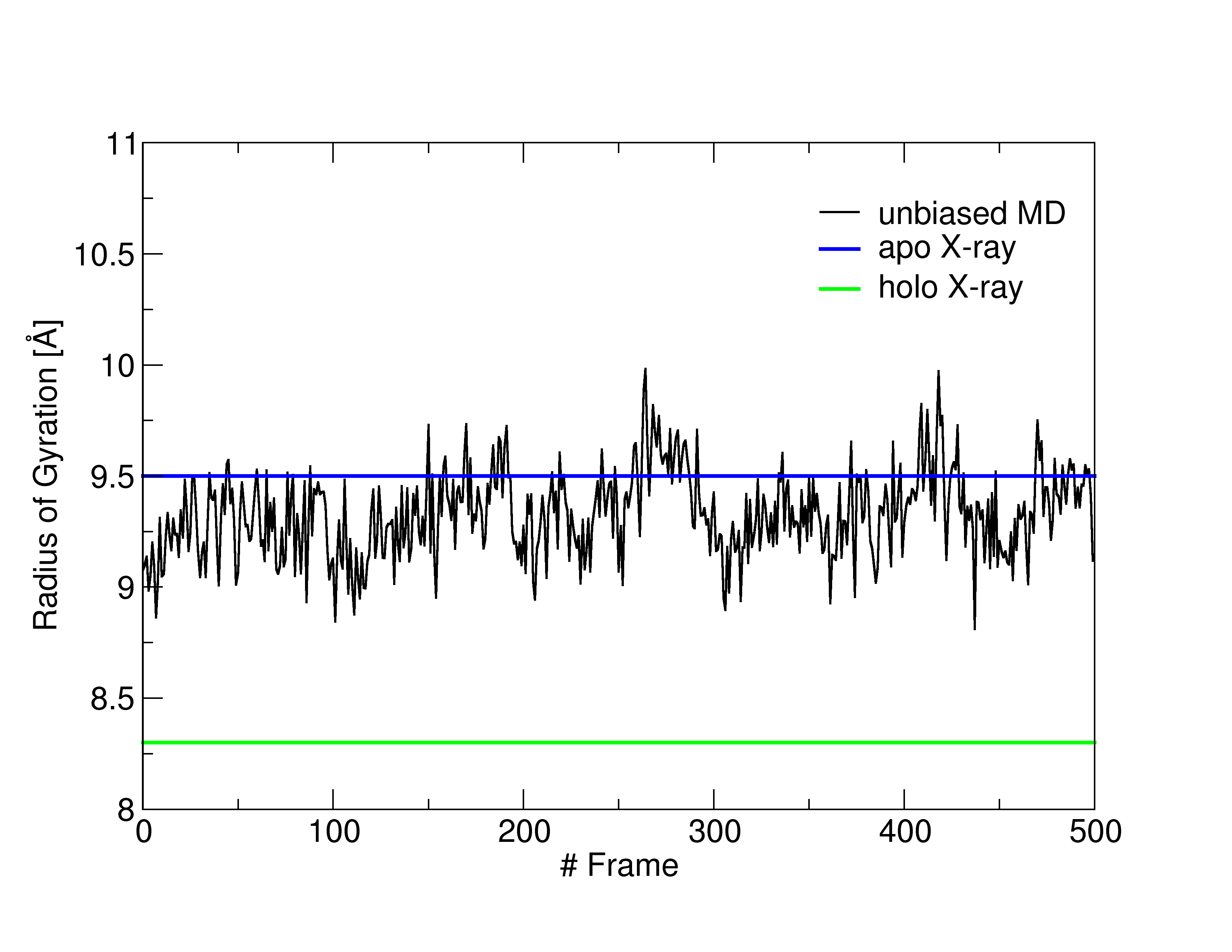
For research purposes these analyses should be performed over longer trajectories, but it is clear that the RoG did not change significantly during the unbiased MD, and thus it did not get close to the holo value. As such, it could be a good choice for a CV that will enhance the sampling of conformations featuring a more closed pocket.
Now you can close xmgrace and calculate the standard deviation of the RoG over the 500 frames of the sample plain MD trajectory provided in the tutorial files. Do this as you prefer, either by means of a graphics plot program such as xmgrace/gnuplot, or by coding this into a script. Here, we will use the bash script av_std-sel-region.sh which can be found in the directory tutorial_files/scripts.
The script takes as input (in this order):
(i) the name of the file containing the values of the CVs;
(ii) the column corresponding to the CV;
(iii) the first and last rows delimiting the size of the data.
As output, you will see on the terminal the average and standard deviation of the CV corresponding to the selected column. To perform the analysis described above, please first copy the script into your working directory:
cp ~/BioExcel_SS_2024/EDES/tutorial_files/scripts/av_std-sel-region.sh .
and make it executable:
chmod +x av_std-sel-region.sh
Then calculate the standard deviations for all the 4 CVs by typing the following command containing a for cycle over the CVs in the file COLVAR_apoMD:
for i in {2..5}; do ./av_std-sel-region.sh COLVAR_apoMD $i 2 501; done
The standard deviations of the CVs will be used to set up the metadynamics run. You should have obtained standard deviations respectively of 0.19, 10.31, 9.81 and 9.69 for the RoG and for the three CIPs (cv1 and cv2-3-4 in plumed-common.dat file).
To setup a bias exchange metadynamics simulation (BE-META), together with the plumed-common.dat file we need four additional files (plumed.X.dat, with X=0,1,2,3), one for each replica that we want to run. As already mentioned, the latter files will contain the instructions to read the plumed-common.dat file, as well as the information on the bias to be applied to the related CV (such as its height and width). Detailed information on all necessary settings to properly run a metadynamics simulation can be found at the following webpages:
As for the tutorial, you can copy all the needed files in the folder where you'll run the simulation:
cp -r ~/BioExcel_SS_2024/EDES/tutorial_files/meta/* ~/BioExcel_SS_2024/EDES/MD/meta/
To run a multi-replica simulation (as it is the case here), GROMACS requires a folder for each replica, containing all the files needed to run the simulations.
Thus, by inspecting the meta folder you will see 4 sub-folders (rep0, rep1, rep2, rep3), one for each replica:
cd ~/BioExcel_SS_2024/EDES/MD/meta
ls
Moving into the rep0 sub-folder and listing its content:
cd rep0
ls
You will find:
(i) a GROMACS input file (tpr extension);
(ii) the plumed-common.dat file;
(iii) a file named plumed.0.dat.
It is instructive to first open and inspect both the data files (.dat extension) to understand the instructions they contain.
First, let's inspect first the plumed-common.dat in this folder, that you will use for running the simulation. Remember that you also edited this file on your own during the second part of this tutorial. Compare the two: is there any difference?
Now open the file plumed.0.dat. First, note the flag "ARG", specifying the CV to which the file refers. In this case you will read "ARG=cv1", meaning that the bias defined in this file will be applied to the CV named "cv1" in the plumed-common.dat file. In our case we defined "cv1" as the radius of gyration.
At this point, you should insert in this file the value for the width of the hills (in the "SIGMA" field). For each CV, we know we should insert a value between 1/4 and 1/2 of the corresponding standard deviation calculated with the av_std-sel-region.sh script.
Note: please keep in mind that smaller values of this parameter are associated to a finer and safer sampling, but also to a longer simulation time to fill up free energy minima and allow the system to efficiently explore the conformational space.
Repeat the above steps for the remaining PLUMED files (plumed.1.dat, plumed.2.dat, plumed.3.dat) within the sub-directories meta/rep1, meta/rep2, meta/rep3.
Before running the simulation, remember to load the GROMACS engine if you haven't done it before:
source /usr/local/gromacs-2023.4_GNU_MPI/bin/GMXRC
Now you are ready to start the metadynamics simulation. Go in the parent meta folder and type the following command:
mpirun -np 4 --hostfile host gmx_mpi mdrun -multidir rep0 rep1 rep2 rep3 -s topol -deffnm BE_GLUCO -plumed plumed.dat -replex 10000 -nsteps 500000000
Where the flag “-replex” is used to specify the frequency (in number of steps) of attempts to exchange the bias between two replicas (for details on all the other flags used, please refer to the official GROMACS documentation available here and here).
Note also the usage of the flag --hostfile for mpirun. It tells the engine to read the file host (in your current directory) containing just the instruction localhost slots=4, telling mpirun to start 4 processes on the same CPU. You can check this page for further details.
If the simulation started without any error message, please wait for about 5 minutes (grab a coffee in the meanwhile :)) and then stop it by pressing CTRL+X or Command [windows symbol] +C. Now, check inside one of the sub-folder (meta/repX) if the file COLVAR.X has been written. For example, considering the first replica (rep0), you can check by typing:
cat rep0/COLVAR.0
If the simulation started correctly, the output should look like the following one (apart from the specific values of the CVs which may be slighly different):
#! FIELDS time cv1 cv2 cv3 cv4
 0.000000 9.159872 201.597309 145.394721 209.429076
 0.002000 9.143103 201.319565 139.480349 213.196953
 0.004000 9.163660 200.618678 145.780933 209.457096
 0.006000 9.110115 206.329567 145.636428 216.329878
 0.008000 9.077969 207.787620 149.916458 219.022940
 0.010000 9.160759 199.164889 151.262484 211.870122
 0.012000 9.169692 197.911613 149.513387 210.555792
 ...
Where you can see that the values of the four CVs (columns 2 to 5) are being written in the file at fixed time intervals (column 1).
If the file has not been written, or it appears to be empty, it means that something likely went wrong (first, check the log file). In this case, in a real scenario, the first thing to do would be to check if the PLUMED input files have been correctly edited and that they are available in each of the sub-folders for the different replicas.
For the sake of finishing the tutorial, in the next and final part we are going to use pre-calculated data.
Go to the SECOND part of the Tutorial Go to the FOURTH part of the Tutorial
[1]: Laio et al., J. Phys. Chem. B, 2005, 109 (14), pp 6714-6721
[2]: Gervasio et al., J Am Chem Soc. 2005 Mar 2;127(8):2600-7
[3]: Vargiu et al., Nucleic Acids Res. 2008 Oct; 36(18): 5910-5921