Enhanced Sampling of Binding Pocket Volume and Shape (tutorial) [Part 4/4]

Go to the THIRD part of the Tutorial

Analyzing the metadynamics simulation

In this section, we are going to evaluate the enhancement of "breathing motions" of the BS (in terms of RoG oscillations, as for the unbiased MD) during metadynamics simulation with our set of EDES CVs. Let's extract the values of the CVs from the trajectory with the tool driver fed by the same input file used for the unbiased run.

Copy the plumed_driver.dat file in your current directory:

cp ../../tutorial_files/Driver/plumed_driver.dat .

Open it with your favourite text editor (e.g. emacs -nw plumed_driver.dat) and scroll down to the end of the file; you should read the following instruction:

...
...
PRINT ARG=cv1,cv2,cv3,cv4 STRIDE=1 FILE=COLVAR_apoMD

Change the name in the "FILE" field, from "COLVAR_apoMD" to "COLVAR_bemeta", save and close the file.

To run driver, type the following command (remember to check for extra spaces and/or to delete and write again the two minus signs before the mf_dcd and plumed flags, if by copying/pasting the previous command doesn’t work):

plumed driver --mf_dcd ../../tutorial_files/bemeta/bemeta_500frames.dcd --plumed plumed_driver.dat

Next, puts the RoG values in a text file with the following command:

awk '(NR >1) {print $2}' COLVAR_bemeta > RoG.dat

Finally, compare the RoG profiles produced by the unbiased and by the metadynamics run with the experimental values (you prepared the ref.dat file containing RoG values of the apo and holo proteins when analyzing the unbiased trajectory; you can also copy the file available in the tutorial_files/apoMD folder, as we'll do here):

xmgrace -nxy ../../tutorial_files/apoMD/ref.dat ../../tutorial_files/apoMD/RoG.dat RoG.dat

You should see a graph like that in Figure 1.

Figure 1: The RoG of the structures sampled during the apoMD simulation (black line) and the metadynamics run (red line). The blue and green lines refer, respectively, to the experimental RoG values in the unbound (apo) and bound (holo) structures.

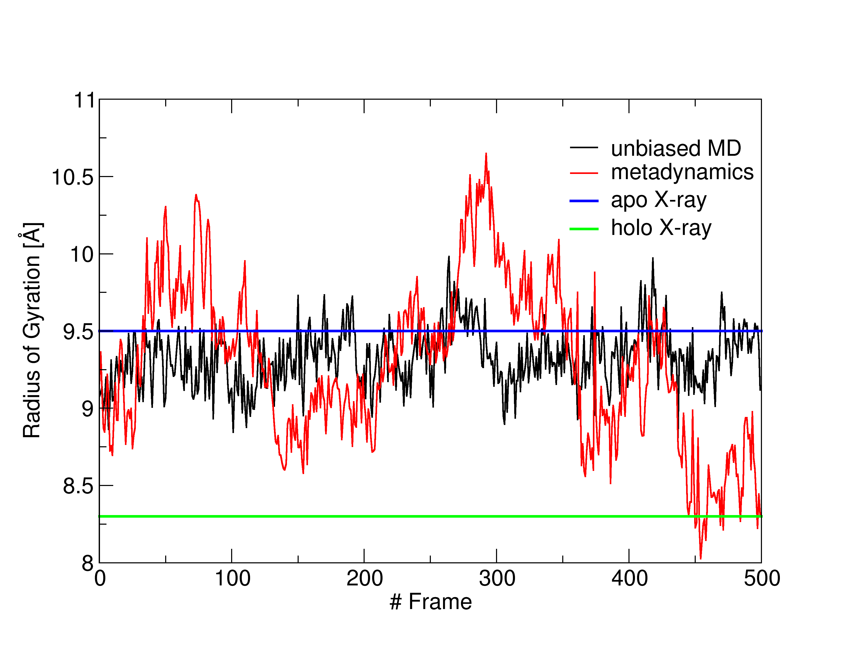
Despite the short simulation time, it is clear that our approach enhances the sampling of conformations with smaller (shrunk BS) and larger (expanded BS) RoG values with respect to the unbiased MD simulation. In particular, around the 300^th and 450^th frames, the system explores conformations displaying a RoG of 10.5 and 8 Å, respectively.

Further imposition of soft restraints on one or more CVs can effectively guide the sampling towards specific regions of the CV-space (check the PLUMED manual for additional details). We followed this strategy in [2].

Cluster analysis

In order to perform ensemble-docking calculations in a reasonable amount of time, it is customary to consider only a limited number of conformations of the target protein. A widely used technique to extract these conformations is the so-called_cluster analysis_ (C.A.) [1].
For our purposes, it is desirable that the C.A. will provide conformations maximizing the structural diversity, particular at the BS. This will improve the probability that, if conformations prone to host the ligand were sampled during the MD run, some near-native structures will be included in the pool of representative clusters selected. The description of strategies developed to achieve this goal is out of the scope of this tutorial, and here we'll perform a C.A. using the RMSD metrics and the GROMOS algorithm (described in ) implemented in GROMACS (for further details, see Daura et al., Angew. Chem. Int. Ed. 1999, 38:236-240 and the GROMACS clustering manual page) and based on the RMSD metrics (the parameter measuring the average distance between different structures).
However, many clustering strategies do exist, often based on different metrics than the RMSD. For example, in [2] we performed a multi-step cluster analysis using the Euclidean distance in the CVs-space.

In order to perform the C.A., copy the file apo_GLUCO_Hs.ndx from ../../tutorial_files/apoMD/ in the MD/meta directory. From the latter, type:

cp ../../tutorial_files/apoMD/apo_GLUCO_Hs.ndx .

This is an index file (made with the make_ndx GROMACS tool) containing the serial numbers of different groups of atoms. Examples of these groups include the whole system, only the protein (without water molecules and ions), water molecules, etc. We'll use the index file to include (inserting them by hand, after generating the file with the GROMACS tool) the serials of binding site region.
The latter with the aim to use it to restrict the clustering calculations only to the BS region.

If you now open the apo_GLUCO_Hs.ndx file with your favourite text editor and scroll down to the end of the file, you'll see the serials of the BS region as reported below.

[ BS ]

280 282 284 286 290 294 295 3084 3086 3089 3090 3091 3093
3095 3098 3100 3101 3122 3124 3126 3129 [...] 4384 4387
4390 4393 4395 4396 4399 4402 4403 4444 4446 4448 4451
4454 4455 4456 4457 4458

Now you can run the cluster analysis using the tool cluster as follows:

gmx_mpi cluster -f ../../tutorial_files/bemeta/bemeta_500frames.trr -s ../../tutorial_files/apoMD/apo_GLUCO_Hs.pdb -n apo_GLUCO_Hs.ndx -cl clusters.pdb -cutoff 0.15 -method gromos -g

Note that we selected an arbitrary RMSD cut-off radius of 0.15 nm (1.5 Å), as criterion to identify two different structures. Details on all the flags can be found in the GROMACS manual.

The following output will appear, asking you to select the specific region of the system that you want to consider. Clearly, as we want to maximize the diversity of BS shapes, we'll perform a C.A. only considering this region:

Select group for least squares fit and RMSD calculation:

Group     0 (         System) has  5773 elements
Group     1 (        Protein) has  5773 elements
Group     2 (      Protein-H) has  2870 elements
Group     3 (        C-alpha) has   351 elements
Group     4 (       Backbone) has  1053 elements
Group     5 (      MainChain) has  1405 elements
Group     6 (   MainChain+Cb) has  1743 elements
Group     7 (    MainChain+H) has  1746 elements
Group     8 (      SideChain) has  4027 elements
Group     9 (    SideChain-H) has  1465 elements
Group    10 (             BS) has    99 elements

Type '10' to restrict the analysis on the BS region. Another message will appear, asking you to select the region you want to save in the pdb file. In this case, the most natural choice is to save the whole protein (identified by Group "1").

Select group for output:

Group     0 (         System) has  5773 elements
Group     1 (        Protein) has  5773 elements
Group     2 (      Protein-H) has  2870 elements
Group     3 (        C-alpha) has   351 elements
Group     4 (       Backbone) has  1053 elements
Group     5 (      MainChain) has  1405 elements
Group     6 (   MainChain+Cb) has  1743 elements
Group     7 (    MainChain+H) has  1746 elements
Group     8 (      SideChain) has  4027 elements
Group     9 (    SideChain-H) has  1465 elements
Group    10 (             BS) has    99 elements

Within a few minutes the program will generate a file named "clusters.pdb", containing the structures of the clusters extracted. Moreover, it should also produce a file named "cluster.log" containing some useful information related to the clustering process. In particular, the first lines should look like the following ones:

Using gromos method for clustering
Using RMSD cutoff 0.15 nm
The RMSD ranges from 0.0477334 to 0.451064 nm
Average RMSD is 0.219825
Number of structures for matrix 500
Energy of the matrix is 4.02515.

Found 14 clusters

Writing middle structure for each cluster to clusters.pdb

...

The software reports on the clustering method selected together with the RMSD cut-off radius and provides some information on the RMSD of the selected region (the BS in our case) among the different conformations. Note that it also specifies the number of clusters that are going to be extracted (14 in our case).

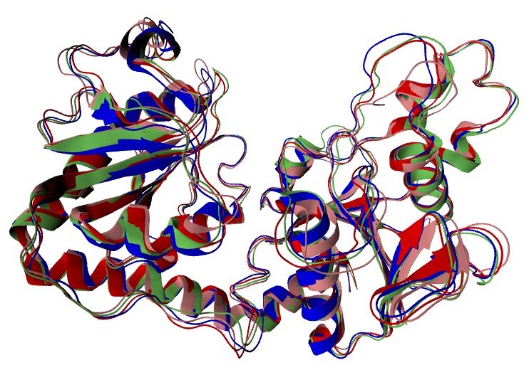
Some of the generated clusters are represented in Figure 1. You can now use your favourite molecular visualization software to open the clusters by your own and check their structural similarity to the true holo geometry, in terms of the conformation of both the whole protein and the BS (e.g. by means of an RMSD analysis). Clearly, for ensemble-docking applications, the clusters should contain at least one structure very similar to the true holo conformation, in particular at the BS. As a rule of thumb, structures displaying an RMSD_BS < 2 Å with respect the holo conformation are said to be "good models" featuring a well-reproduced BS.

Figure 1: The conformations of 4 out of the 14 clusters extrated using a RMSD cut-off radius of 1.5 Å. The structures are represented with VMD in different colors and using "New Cartoon" as drawing method.

Congratulations!
This was the last step of the tutorial. In case you are interested in using these clusters for ensemble-docking applications, you can refer to the extended version of the tutorial, containing also the docking part performed with HADDOCK , the software developed by the Structural Biology Group @ Utrecht University led by Prof. A. Bonvin.

References

[1]: Shao et al., J. Chem. Theory Comput. 2007, 3, 2312-2334

[2]: Basciu A. et al., J. Chem. Inf. Model. 2019, 59, 4, 1515-1528