python with conda
A very short guide for installing python packages (pymol in this example) as a non-privileged
| Molecular Modeling Lab |
Go to the FIRST part of the Tutorial Go to the THIRD part of the Tutorial
We are going to perform metadynamics simulations using GROMACS and PLUMED, a plugin facilitating the implementation of different enhanced sampling techniques in several simulation packages. Metadynamics, developed in 2000 by Laio and Parrinello [1], enforces systems to escape free energy minima by means of a history-dependent fictitious potential, pushing it to explore conformations associated to other (meta)stable basins and/or free energy barriers. This is achieved by defining a set of collective variables (CVs, e.g. a distance, an angle, the number of contacts between two groups of atoms, etc.) identifying the relevant (slow) motions to be enhanced in order to steer the sampling of rare conformations. On the CV-space are then deposited a number of Gaussian-like potentials (hills), whose effect is transmitted to the real atoms of the system, thus enhancing the conformational sampling. The choice of the CVs is fundamental: a good CV should be associated with a slow motion of the system (in absence of bias), so that its value at conformations associated with different free energy basins will differ too. Rules of thumbs to guide the choice of the height, width and deposition time of the hills have been outlined over the years [2,3]. Since its introduction, many flavors of metadynamics were developed [4] (whose description is out of the scope of this tutorial). Here we will use the so-called "well tempered metadynamics" [5], that represents an improvement over the original algorithm due to the possibility of focusing on regions of the free energy surface that are physically meaningful to explore.
Often a single CV is not sufficient to catch the relevant slow motions associated to a process of interest. Indeed, all the CV-based methods often exploit the use of multiple variables, which ideally should be orthogonal to each other so as to enhance the sampling along independent directions of the CV space. In the metadynamics world, a clever method to enhance sampling across a set of multiple CVs is the so called "bias-exchange metadynamics" [5]. With this approach, multiple simulations of the system at the same temperature are performed, biasing each replica with a time-dependent potential added to a different CV. Exchanges between the bias potentials on the different variables are periodically attempted according to a Metropolis criterion.
We are going to perform a bias-exchange well-tempered metadynamics simulation using PLUMED. The first step is thus to define the CVs in the PLUMED input file. Here we will enhance the conformational sampling at the binding site (BS) of the apo-form of GLUCO, by biasing specific CVs related to the BS. Note that this is clearly not the only possible choice, as, for example, one may wish to include also CVs defined over the whole protein.
To define the BS, we exploit the crystallographic structure of the GLUCO-UDP complex. Namely we define the BS as the site lined by all residues having at least one atom within 3.5 Å from the ligand UDP. From the RCBS pdb databank we first download the bound form of the protein (PDB ID: 1JG6) in the Xray directory. You can do it either with a browser or directly from the terminal. In the latter case, you can use the command wget inside the Xray directory as follows:
cd Xray
wget https://files.rcsb.org/download/1JG6.pdb
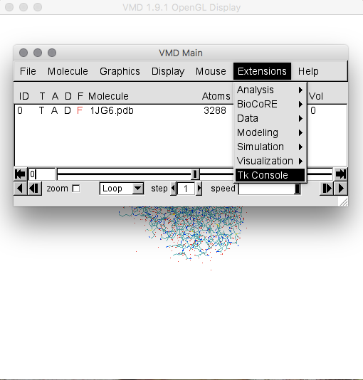
Using VMD it is possible to visualize the BS and get the resid IDs (hereafter named "res IDs") of all residues lining the site (each ID is a number associated to the position of a specific residue in the protein chain) and other useful information about the site. To open the PDB with VMD:
vmd 1JG6.pdb
You will see the VMD main window, as well as the "Display" and "Graphics" windows. Go to the "Extensions" menu and select the "Tk Console" (Figure 1; for details on VMD syntax, see the VMD manual).
Within the Tk Console, the following commands allow to define the BS and extract the resIDs (Figure 2):
set BS_residues [atomselect top "protein and same residue as within 3.5 of resname UDP and noh"]
lsort -integer -uniq [$BS_residues get resid]
If you copy these commands in the Tk console, please make sure that you don't include any extra space in them.
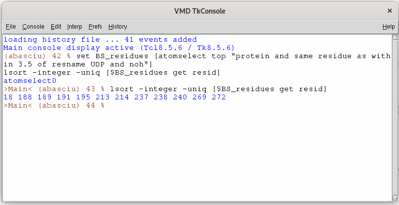
So, while the first command defines the binding site, the second one will print the list of resIDs lining that site.
The list of resIDs obtained by the previous commands should be:
18 188 189 191 195 213 214 237 238 240 269 272
As specified above we selected all protein residues with at least one atom within 3.5 Å from the experimental ligand in the bound (holo) structure (the UDP molecule in this case). However, for cases in which no structure with the co-crystallized ligand is available a similar procedure will not be feasible. A possible solution could be the usage of a binding-site detection software among the plethora available (such as COACH).
In particular, in [6,7] we show how the BS selection according to the COACH software is virtually identical to the one obtained by using the holo structure.
Another useful parameter we can extract from the experimental structure of the holo protein is the radius of gyration (RoG) of the BS, which indicates its compactness. This is relevant as larger values of the RoG should correspond to more open conformations of the BS. Since the binding of a small ligand to the BS of a protein often causes a partial collapse of the pocket, we expect the RoG of the holo to be smaller than that of the apo protein. We can calculate the value of the RoG of the BS in the experimental structure in VMD typing the following command in the Tk Console:
measure rgyr $BS_residues
You should get the value of 8.29 Å. We'll use this value later. Now you can close VMD (if you opened it from the terminal, simply digit "quit") as we will reopen it in another folder.
When running a metadynamics simulation with PLUMED, CVs should be defined using the atomic serial numbers (and not the residue IDs); thus, we must extract the serial numbers from the list of residues. We do it in VMD by loading either a ".gro", a ".pdb", or any other structure file, as long as the topology matches the one of the system you are going to simulate.
Here you are going to use a "pdb" file of the protein we will be simulating (the unbound conformation) available in the tutorial_files directory.
Now go to the ../MD/plain directory, copy there the apo_GLUCO_Hs.pdb file from the ../../tutorial_files/apoMD folder, and open it on VMD:
cd ../MD/plain
cp ../../tutorial_files/apoMD/apo_GLUCO_Hs.pdb .
vmd apo_GLUCO_Hs.pdb
Note that the apo_GLUCO_Hs.pdb structure has been hydrogenated, as the atom numbering (serials) of residues should match with the one of the structure we will be simulating.
Open now the Tk console and paste therein all the following commands that will define a selection of the BS, calculate its RoG, and get the list of serial numbers lining the site:
set BS [atomselect top "protein and resid 18 188 189 191 195 213 214 237 238 240 269 272 and noh"]
measure rgyr $BS
lsort -integer -uniq [$BS get serial]
Note that the addition of "and noh" in the BS definition is used to avoid getting also the serial numbers of hydrogen atoms, which would increase the computational cost of the simulation significantly.
Before going on, spend some time to make sure you understand the aim of each one of the previous commands. Note that we also calculated the value of the RoG of the BS for the apo structure (9.46 Å), as we need this value later. By comparing the RoG of the apo with the one of the holo (8.29 Å) we detect an overall decrease of 12% along the apo-to-holo structural transition.
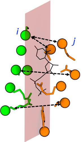
The RoG of the BS, which is one of the CVs in EDES, is exploited to enhance shrinking/expansion of the site (associated to small and large values of the RoG, respectively). The three additional CVs used to bias the simulation are the three (pseudo)contacts across the inertia planes (CIPs), each one defined as the number of contacts between residues of the BS on opposite sides of the corresponding inertia plane. As demonstrated in [6], these CVs provide a computationally cheap way to induce fluctuations in the shape of the BS along each of the three orthogonal spatial directions.
To define the CIPs we will use a tcl script based on the "Orient" package for VMD, which implements the following procedure:
Calculates the principal axes of inertia (x,y,z) of the BS;
Defines, for each couple of axes, a plane passing through the center of mass of the BS and orthogonal to the third direction (e.g. xy plane ortoghonal to the z-axis);
Splits the residues lining the BS in two lists along each direction, according to their position with respect to each plane. In particular, the position of each residue will be identified by the center of mass of its backbone atoms.
The resulting 6 lists (2 for each of the 3 planes) These lists will be used to define the 3 additional CVs (CIPs) used in metadynamics simulation.
The script requires: (i) the list of residues lining the BS and (ii) the protein structure.
To simplify the tutorial, here the list of BS residues is defined within the script itself. You should already have the "apo_GLUCO_Hs.pdb" file open in VMD. If not, open it again (vmd apo_GLUCO_Hs.pdb), then load the divide_into_lists.tcl script described above within the Tk console:
source ~/BioExcel_SS_2024/EDES/tutorial_files/scripts/divide_into_lists.tcl
If the script doesn't work, open it with your favourite text editor and check if the path of the Orient and la1.0 packages (in the first two lines) is correct.
The output in the Tk console window should look like this:
plane xy
Z_1 resids: 18 237 238 240 269 272
Z_2 resids: 188 189 191 195 213 214

Z_1 serials:
280,282,294,295,3877,3879,3897,3898,3899,3901,3916,3917,3932,3934,3947,
3948,4380,4382,4402,4403,4444,4446,4457,4458

Z_2 serials:
3084,3086,3089,3090,3091,3093,3100,3101,3122,3124,3144,3145,3181,3183,
3203,3204,3480,3482,3498,3499,3500,3502,3505,3506

plane xz
Y_1 resids: 195 269 272
Y_2 resids: 18 188 189 191 213 214 237 238 240

Y_1 serials:
3181,3183,3203,3204,4380,4382,4402,4403,4444,4446,4457,4458

Y_2 serials:
280,282,294,295,3084,3086,3089,3090,3091,3093,3100,3101,3122,3124,
3144,3145,3480,3482,3498,3499,3500,3502,3505,3506,3877,3879,3897,
3898,3899,3901,3916,3917,3932,3934,3947,3948

plane yz
X_1 resids: 188 189 195 213 214 237 238 272
X_2 resids: 18 191 240 269

X_1 serials:
3084,3086,3089,3090,3091,3093,3100,3101,3181,3183,3203,3204,3480,
3482,3498,3499,3500,3502,3505,3506,3877,3879,3897,3898,3899,3901,
3916,3917,4444,4446,4457,4458

X_2 serials:
280,282,294,295,3122,3124,3144,3145,3932,3934,3947,3948,4380,4382,
4402,4403
As anticipated above, for each of the three planes this tcl script gives the lists of residues and serials defining the groups of (heavy) atoms lying on opposite sides of each inertia plane. A graphical example of such classification is shown in Figure 3.
Cross-check that the topology file used to extract the serial numbers is identical to the one of the protein to be simulated. This is to avoid mismatching between the serial numbers corresponding, for example, to hydrogenated and non-hydrogenated structures;
Visually inspect (for example with VMD or Pymol) how the residues are distributed within the BS to possibly optimize by hand the definition of the three CVs related to inertia planes. For example, it is better to avoid that residues belonging to the same secondary-structure element and very close in space belong to different lists.
In this example the topology file and the definition of the lists have been already checked and no further inspection is required. You can now close VMD.
After extracting the serial numbers defining all the CVs it is finally possible to fill the PLUMED input files and run the metadynamics simulation. You are now asked to make the first of these files, named plumed-common.dat, which basically contains the definition of CVs.
The first line of this file (shown at the bottom of this page) defines the length/energy/time units to be used during the simulation and the second one allows for the bias exchanges between replicas (crucial ingredient of the bias-exchange approach). Then, the file contains the definition of the CVs. The first one, the radius of gyration of the BS has been already defined in the example shown below, as well as the first one of the three CIP variables.
You should now complete the file "plumed-common.dat" by defining the remaining two CIP variables. To do so, just check how the first one (cv2) has been defined and apply the same scheme to define the others. Note that the only difference regards the splitting of the BS residues into two lists (GROUPA and GROUPB) that are different across different inertia planes.
Open a file named "plumed-common.dat" with your favourite text editor, copy there the part of the file which has already been prepared (shown below) and complete it with what is missing.
You can safely close VMD as the output of the divide_into_lists.tcl script is available on this page.
If you need further information about how to define the CVs, please refer to the PLUMED manual. In particular, spend some time reading the documentations about how to define the CVs we'll be using in this tutorial:
Please find below the scheme of the "plumed-common.dat" file to be completed.
Note that R_0, which indicates the value at which the switching function representing the coordination number has the value 0.5 (half maximum), must be added to every CIP CV.
Once done, you can go to the third part of this tutorial, where we will make the remaining PLUMED input files and run the simulation.
# plumed-common.dat
# YOU HAVE TO COMPLETE THIS FILE!

# Note: Remove all the extra spaces at the end of the lines
# containing the serials.


UNITS LENGTH=A ENERGY=kcal/mol TIME=ns
RANDOM_EXCHANGES

#RoG BS
cv1: GYRATION TYPE=RADIUS ATOMS=280,282,284,286,290,294,
295,3084,3086,3089,3090,3091,3093,3095,3098,3100,3101,
3122,3124,3126,3129,3132,3135,3137,3138,3141,3144,3145,
3181,3183,3185,3188,3191,3194,3196,3197,3200,3203,3204,
3480,3482,3484,3487,3488,3490,3492,3494,3496,3498,3499,
3500,3502,3505,3506,3877,3879,3881,3884,3887,3890,3893,
3897,3898,3899,3901,3903,3905,3909,3912,3916,3917,3932,
3934,3936,3939,3942,3943,3947,3948,4380,4382,4384,4387,
4390,4393,4395,4396,4399,4402,4403,4444,4446,4448,4451,
4454,4455,4456,4457,4458


##### CIPs

### Plane XY [along the Z-axis]

cv2: COORDINATION GROUPA=280,282,294,295,3877,3879,3897,3898,3899,
3901,3916,3917,3932,3934,3947,3948,4380,4382,4402,4403,4444,4446,
4457,4458 GROUPB=3084,3086,3089,3090,3091,3093,3100,3101,3122,3124,
3144,3145,3181,3183,3203,3204,3480,3482,3498,3499,3500,3502,3505,
3506 R_0=12.0

### Plane XZ [along the Y-axis]

cv3:

### Plane YZ [along the X-axis]

cv4:
Go to the FIRST part of the Tutorial Go to the THIRD part the Tutorial
[1]: Laio and Parrinello, PNAS October 1, 2002. 99 (20) 12562-12566
[2]: Deserno and Holm, J. Chem. Phys. 109, (1998) 7678
[3]: Laio et al., J. Phys. Chem. B, 2005, 109 (14), 6714-6721
[4]: Laio and Gervasio, Reports on Progress in Physics (2008), Vol 71, Num 12
[5]: Barducci et al., Phys. Rev. Lett. 2008, 100, 020603
[6]: Basciu et al., J Chem. Inf. Model 2019, 59 (4), 1515–1528
[7]: Basciu et al., 2024, DOI:10.1101/2024.06.02.597018