Enhanced Sampling of Binding Pocket Volume and Shape (tutorial) [Part 1/4]

Introduction

---

In this tutorial we will exploit enhanced sampling molecular dynamics (MD), namely metadynamics [1], to improve the sampling of bound-like (holo) conformations of a protein starting from its unbound (apo) one. This is a central problem in computational biology and it has a clear impact on Computer-Aided Drug Design (CADD) efforts [2,3,4,5], in particular at the steps involving molecular docking calculations [2].
Concerning molecular docking, the calculations can be grossly divided into the two following tasks:

• Search for putative binding poses of the ligand (potential drug candidate) onto a region (binding site) of the selected protein target(s);

• Rank all generated poses according to a "scoring function" that should ideally reproduce at best the free energy of binding of the complex. While such a matching can be questioned, scoring functions are routinely employed to sort the poses in a way to distinguish between the stable and unstable ones.

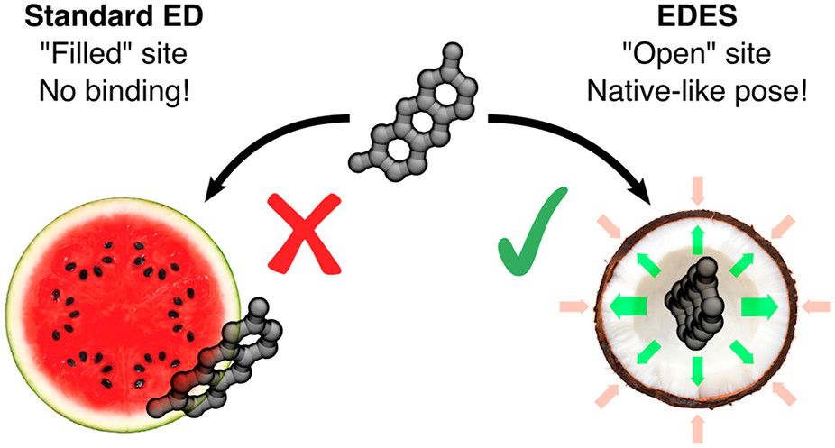
In this tutorial we will see how to generate bound-like protein conformations according to the EDES workflow (A. Basciu, G. Malloci, F. Pietrucci, A.M.J.J. Bonvin, A.V. Vargiu, Holo-like and Druggable Protein Conformations from Enhanced Sampling of Binding Pocket Volume and Shape, J. Chem. Inf. Model, 2019, 59, 4, 1515-1528).

Readers interested in using these conformations in ensemble docking calculations should refer to the extended (but older) version of the tutorial, where we use the docking software HADDOCK.
The docking step will not be addressed in this tutorial.

---

Requirements

The following software packages will be used for this tutorial:

• GROMACS: a versatile package to perform MD simulations and related analyses;

• PLUMED: a package working with different MD simulation engines used to implement different flavours of non-equilibrium MD simulations (among the others features), as well as for MD analysis purposes;

• VMD: a molecular visualization tool allowing to perform a number of calculations analyses on MD trajectories and single structure files (such as pdb and gro files);

• XMGRACE: a friendly 2D plotting tool, allowing also to perform a number of statistical analyses on the data;

• Emacs: a terminal-based text editor, among the plethora available. Feel free to use a different one if you prefer.

However, the tutorial can be performed also using a different version of GROMACS or another MD engine, as long as it supports the PLUMED package. Check the PLUMED page to see the MD engines supporting PLUMED. Note that different MD engines or PLUMED versions might need different commands.

---

System setup and MD simulations

First, open a terminal in your home directory, go into the "~/BioExcel_SS_2023" folder and create the "EDES" directory there. In case you don't have that folder in your workstation, remember to create it. Then, inside the "EDES" folder, create the subfolders needed for the tutorial: one for the Xray structures, one for the plain MD simulation and one for the metadynamics run.

cd ~/BioExcel_SS_2023
mkdir EDES
cd EDES
mkdir -p Xray MD/plain/analysis MD/meta

To run this tutorial you will need some pre-calculated data and scripts, that can be downloaded here (compressed, ~150 MB).

You can download the archive with your browser or via the wget command as follows:

wget "https://unicadrsi-my.sharepoint.com/:u:/g/personal/attiliov_vargiu_unica_it/EUz0MevZkGhLv5gGzR9qcVIB-f6y10LDYZng7qqRrOFblg?e=FUpeb8&download=1" -O tutorial_files.tar.gz

Now extract the archive with the command: tar xvzf tutorial_files.tar.gz.
Before going on, make sure you have a folder name tutorial_files in the EDES directory.

Setting up the simulation system

NOTE: if you are running the tutorial in a terminal with loaded conda scripts, better to deactivate everything and load the source files of GROMACS (and PLUMED) to avoid compatibility issues. Follow the instructions below (work for our machines):

conda deactivate
source /home/utente/.plumedrc
source /usr/local/gromacs_2022_3/bin/GMXRC

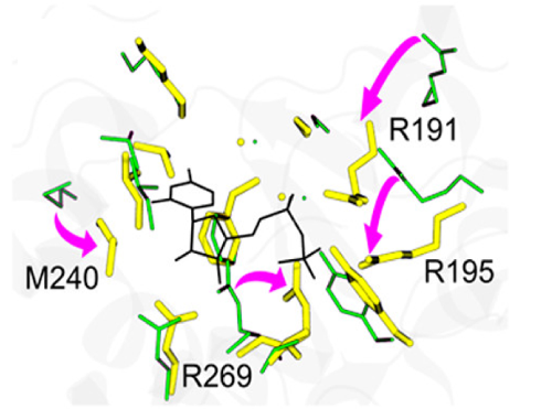
Our target protein is the T4 phage beta-glucosyltransferase (hereafter GLUCO), which displays large binding site (BS) distortions (~ 2.8 Å) upon binding to one of its physiological ligands (uridine diposphate - UDP) (Figure 1). You can find a simple pymol session of the structures of apo and holo here. To visualize it, type:

pymol /home/utente/Scaricati/BE_gluco_apo_holo.pse

Importantly, proteins displaying large conformational changes between their unbound and bound structures are generally challenging targets for molecular docking programs.

Figure 1: GLUCO's binding site. In green and yellow, respectively, the BS residues in the unbound (apo) and bound (holo) experimental structure. The ligand (UDP) is also shown with black lines for reference. Magenta arrows highlight residues undergoing the largest conformational change in the apo-to-holo transition.

To run a metadynamics simulation with GROMACS, you need:

• The GROMACS input file, a binary file containing all the information needed to run the MD calculations. This file will be generated by the grompp command, which needs both the structure and topology files together with an MD input file containing the instructions to run the simulation (simulation type, pressure and temperature control flags, treatment of long-range interaction, information to be printed, etc...);

• The PLUMED input files, used to actually run the metadynamics. These files contain the definition of the collective variables (CVs) as well as additional parameters such as the height and the width of energy hills to be deposited, etc.

Making the GROMACS input file

As this tutorial will focus on metadynamics simulations, we will not cover the preparation of a GROMACS input file, limiting ourselves to a brief conceptual outline (for further details please refer to the GROMACS manual [6] and to the GROMACS tutorial of this school):

• Download the PDB file of the unbound X-ray protein structure (PDB ID: 1JEJ);
• With your favorite text editor check the PDB file for missing residues. If needed, remove the crystallographic water molecules from the file;
• Generate a topology file (top extension) containing information on atom types, bonded and non-bonded interactions, etc. At this step you will also be asked to choose the force field to use in your simulation;
• Generate a structure file in the native GROMACS format (gro extension) containing the initial protein structure. Since simulations will be performed in explicit solvent, in this step you also need to include water molecules and ions in your simulation box;
• Perform a quick structural relaxation of the system and heat it up to the desired temperature (e.g. 300 K);
• Generate the GROMACS input file (tpr extension) combining the topology and structure files together with the MD input file (mdp extension).

Note that all the above-mentioned steps are explained in detail in the extended (but older) version of the tutorial.

In the next step you will see how to generate the PLUMED input (plain text files) needed to actually run a metadynamics simulation.

Go to the SECOND part of the Tutorial

References

[1]: Laio and Parrinello, PNAS October 1, 2002. 99 (20) 12562-12566

[2]: Huang and Zou, Proteins. 2007 Feb 1;66(2):399-421

[3]: Forli, Molecules 2015, 20, 18732-18758

[4]: Mandal et al., Eur J Pharmacol. 2009 Dec 25;625(1-3):90-100

[5]: Sliwoski et al., Pharmacol Rev. 2013 Dec 31;66(1):334-95

[6]: Pronk et al. Bioinf, 29 (2013), pp. 845-854